Question No. 5 - MMPC-005 - Quantitative Analysis for Managerial Applications - MBA and MBA (Banking & Finance)

Solutions to Assignments

                            MBA and MBA (Banking & Finance)

                    MMPC-005 - Quantitative Analysis for  Managerial 

                                                Applications

Question No. 5. 

Write the short note on any three of the following:- 

(a) Mathematical Property of Median 

The value which occupies the centre position amongst the observations when arranged in ascending or descending order is the median. Fifty per cent scores are above or below the median. Hence, it is named as 50th percentile or positional average. The location of the median is dependent on whether the data set consists of an even or odd number of values. The method of finding the median is different for even and an odd number of observations.

Median Properties

In statistics, the properties of the median are explained in the following points.

• Median is not dependent on all the data values in a dataset.
• The median value is fixed by its position and is not reflected by the individual value.
• The distance between the median and the rest of the values is less than the distance from any other point.
• Every array has a single median.
• Median cannot be manipulated algebraically. It cannot be weighed and combined.
• In a grouping procedure, the median is stable.
• Median is not applicable to qualitative data.
• The values must be grouped and ordered for computation.
• Median can be determined for ratio, interval and ordinal scale.
• Outliers and skewed data have less impact on the median.
• If the distribution is skewed, the median is a better measure when compared to mean.

Formula to Find Median for Discrete Series

Calculating the median for individual series is as follows:

• The data is arranged in ascending or descending order.
• If it is an odd-sized sample, median = value of ([n + 1] / 2)th item.
• If it is an even-sized sample, median = ½ [ value of (n / 2)th item + value of ([n / 2] + 1)th item]

Calculating the median for discrete series is as follows:

• Arrange the data in ascending or descending order.
• The cumulative frequencies need to be computed.
• Median = (n / 2)th term, n refers to cumulative frequency.

The formula for finding the median for a continuous distribution is:

Where l = lower limit of the median class

f = frequency of the median class

N = the sum of all frequencies

i = the width of the median class

C = the cumulative frequency of the class preceding the median class

(b) Decision Tree Approach 

A decision tree is a support tool with a tree-like structure that models probable outcomes, cost of resources, utilities, and possible consequences. Decision trees provide a way to present algorithms with conditional control statements. They include branches that represent decision-making steps that can lead to a favorable result.

The flowchart structure includes internal nodes that represent tests or attributes at each stage. Every branch stands for an outcome for the attributes, while the path from the leaf to the root represents rules for classification.

Decision trees are one of the best forms of learning algorithms based on various learning methods. They boost predictive models with accuracy, ease in interpretation, and stability. The tools are also effective in fitting non-linear relationships since they can solve data-fitting challenges, such as regression and classifications.

Applications of Decision Trees

 

1. Assessing prospective growth opportunities

One of the applications of decision trees involves evaluating prospective growth opportunities for businesses based on historical data. Historical data on sales can be used in decision trees that may lead to making radical changes in the strategy of a business to help aid expansion and growth.

 

2. Using demographic data to find prospective clients

Another application of decision trees is in the use of demographic data to find prospective clients. They can help streamline a marketing budget and make informed decisions on the target market that the business is focused on. In the absence of decision trees, the business may spend its marketing market without a specific demographic in mind, which will affect its overall revenues.

 

3. Serving as a support tool in several fields

Lenders also use decision trees to predict the probability of a customer defaulting on a loan by applying predictive model generation using the client’s past data. The use of a decision tree support tool can help lenders evaluate a customer’s creditworthiness to prevent losses.

Decision trees can also be used in operations research in planning logistics and strategic management. They can help in determining appropriate strategies that will help a company achieve its intended goals. Other fields where decision trees can be applied include engineering, education, law, business, healthcare, and finance.

(c) Stratified vs. Cluster Sampling 

In statistics, two of the most common methods used to obtain samples from a population are cluster sampling and stratified sampling.

This tutorial provides a brief explanation of both sampling methods along with the similarities and differences between them.

Cluster Sampling

Cluster sampling is a type of sampling method in which we split a population into clusters, then randomly select some of the clusters and include all members from those clusters in the sample.

For example, suppose a company that gives whale-watching tours wants to survey its customers. Out of ten tours they give one day, they randomly select four tours and ask every customer about their experience.

Stratified Sampling

Stratified sampling is a type of sampling method in which we split a population into groups, then randomly select some members from each group to be in the sample.

For example, suppose a high school principal wants to conduct a survey to collect the opinions of students. He first splits the students into four stratums based on their grade – Freshman, Sophomore, Junior, and Senior – then selects a simple random sample of 50 students from each grade to be included in the survey.

Cluster sampling and stratified sampling share the following similarities:

- Both methods are examples of probability sampling methods – every member in the population has an equal probability of being selected to be in the sample.

- Both methods divide a population into distinct groups (either clusters or stratums).

- Both methods tend to be quicker and more cost-effective ways of obtaining a sample from a population compared to a simple random sample.

Cluster sampling and stratified sampling share the following differences:

- Cluster sampling divides a population into groups, then includes all members of some randomly chosen groups.

- Stratified sampling divides a population into groups, then includes some members of all of the groups.

(d) Pearson’s Product Moment Correlation Coefficient

The Pearson product-moment correlation coefficient (or Pearson correlation coefficient, for short) is a measure of the strength of a linear association between two variables and is denoted by r. Basically, a Pearson product-moment correlation attempts to draw a line of best fit through the data of two variables, and the Pearson correlation coefficient, r, indicates how far away all these data points are to this line of best fit (i.e., how well the data points fit this new model/line of best fit).

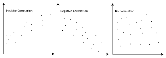
The Pearson correlation coefficient, r, can take a range of values from +1 to -1. A value of 0 indicates that there is no association between the two variables. A value greater than 0 indicates a positive association; that is, as the value of one variable increases, so does the value of the other variable. A value less than 0 indicates a negative association; that is, as the value of one variable increases, the value of the other variable decreases. This is shown in the diagram below:

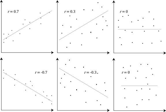
The stronger the association of the two variables, the closer the Pearson correlation coefficient, r, will be to either +1 or -1 depending on whether the relationship is positive or negative, respectively. Achieving a value of +1 or -1 means that all your data points are included on the line of best fit – there are no data points that show any variation away from this line. Values for r between +1 and -1 (for example, r = 0.8 or -0.4) indicate that there is variation around the line of best fit. The closer the value of r to 0 the greater the variation around the line of best fit. Different relationships and their correlation coefficients are shown in the diagram below: